Sunday, April 25, 2010

PythonXY 2.6.2 + Panda3d 1.7.0 + JModelica 1.1b1 – How to get to work together

If Panda3D 1.7.0 is added to Python using a ‘pth’ file, then JModelica 1.1b1 will load the wrong ‘mscvrt.dll’ and fail to initialize. This problem occurs:

In [1]: import jmodelica.examples.cstr as cstr
C:\Python26\lib\site-packages\jpype\_pykeywords.py:18: DeprecationWarning: the s
ets module is deprecated
  import sets
---------------------------------------------------------------------------
OSError                                   Traceback (most recent call last)

C:\JModelica.org-1.1b1\work\<ipython console> in <module>()

C:\JModelica.org-1.1b1\Python\jmodelica\examples\cstr.py in <module>()
      9 from jmodelica.initialization.ipopt import NLPInitialization
     10 from jmodelica.initialization.ipopt import InitializationOptimizer
---> 11 from jmodelica.simulation.sundials import TrajectoryLinearInterpolation
     12 from jmodelica.simulation.sundials import SundialsDAESimulator
     13 from jmodelica.optimization import ipopt

C:\JModelica.org-1.1b1\Python\jmodelica\simulation\sundials.py in <module>()
     14
     15 try:
---> 16     from pysundials import cvodes
     17     from pysundials import ida
     18     from pysundials import nvecserial

C:\Python26\lib\site-packages\pysundials\cvodes.py in <module>()
     38
     39 import ctypes
---> 40 import sundials_core
     41 import nvecserial
     42

C:\Python26\lib\site-packages\pysundials\sundials_core.py in <module>()
     87 f.close()
     88
---> 89 libc = loadlib("c")
     90 try:
     91         libc.fdopen.argtypes = [ctypes.c_int, ctypes.c_int]

C:\Python26\lib\site-packages\pysundials\sundials_core.py in loadlib(libname)
     63                 lib = ctypes.CDLL(libpaths[libname])
     64         except OSError, e:
---> 65                 raise OSError("%s\nCannot load shared library %s. Please
check you config file and ensure the paths to the shared libraries are correct.
"%(e, libpaths[libname]))
     66         return lib
     67

OSError: [Error 1114] A dynamic link library (DLL) initialization routine failed

Cannot load shared library C:\Panda3D-1.7.0\bin\msvcrt.dll. Please check you con
fig file and ensure the paths to the shared libraries are correct.

The occurs in pysundials because the util.find_library('msvcrt') in the ctypes module is attempting to load the ‘msvcrt.dll’ which is installed with Panda3D. This problem can be fixed by forcing pysundials to load a compatible msvcrt.dll file, rather than the most recent. This is done by modifying pysundials_core.py to point to the correct dll. The following change starting at line 42 will force a specific dll to be loaded. The path and dll to use will be specific to each system.

if os.name == "nt":
    #clib = util.find_library('msvcrt')
    clib = 'C:\\Program Files (x86)\\Java\\jdk1.6.0_17\\jre\\bin\\msvcrt.dll'
else:
    clib = util.find_library('c')
An interesting tool - Pyspread

This is an interesting project: Pyspread. It is still a little rough, but shows a lot of promise as a way to use Python. Basically it is a spreadsheet built in Python and using Python to define cell behavior. I’ve installed it under PythonXY and it appears to work. A little slow, but not bad for a beta.

Alternatives to a prototyping tools that make python easier to use are:

In general some alternative environments to prototype behavior include:

Wednesday, April 21, 2010

How to get Panda3D to work with PythonXY

This note applies to Panda3d ver 1.7.0 and PythonXY ver 2.6.2 on a windows system.

  1. Install PythonXY.
  2. Install Panda3D, however do NOT set it as the default python interpreter.
  3. Add a ‘pth’ file to the python site-packages directory. I created a file named panda.pth and saved it at “C:\Python26\Lib\site-packages”. The file had the following contents:

C:/Panda3D-1.7.0
C:/Panda3D-1.7.0/bin

To check that the installation works, use an example from the Panda3D manual.

from direct.showbase.ShowBase import ShowBase
class MyApp(ShowBase):
	def __init__(self):
		ShowBase.__init__(self)
app = MyApp()
app.run()

Wednesday, April 7, 2010

How to fit exponential decay – An example in Python

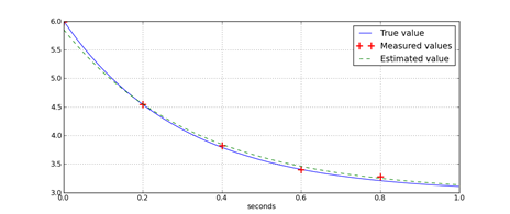
titleGraphOfExponentFit

Linear least squares can be used to fit an exponent. However, the linear least square problem that is formed, has a structure and behavior that requires some careful consideration to fully understand. Usually, fitting is used because the data is noisy. If only the number of data points equal to the number of free variables in system of equations is used, the estimate of parameters will generally be poor.

For example, a common problem is estimating the parameters or coefficients for cooling. For example, a mass is heated to a steady temperature, then left to cool. Ignoring a lot of detail, a model of this behavior can be described by a simple first order, ordinary differential equation:

imageIn this equation, T is the temperature of the object, T0 is the ambient temperature, and h is a coefficient of hear transfer. When T0 is held constant and T(t=0) is not equal to T0, T(t) is described by an exponential decay function.

An exponential decay function is

image

For a system whose behavior can be defined by exponential decay, the parameters for the decay function can be found using least-squares. Since the data usually has measurement errors, the measured data from an exponential decay will usually contain an error term.

imageIdeally, this equation could  be directly set up as a linear least squares problem.   However, minimizing the norm of epsilon, requires solution via methods other than linear least squares. To formulate this problem as a linear least squares minimization, a new error term inside the exponent is introduced, del.

image

The usual way to set this problem up is to minimize the norm of epsilon.

image

However, if the problem is set up to minimize the 2-norm of del, then a linear least squared minimization can be formed.

 image

To linearize this problem, the terms in the constraints are rearranged, the natural log of each side is taken, and the properties of logarithms are isolate terms.

image

The problem statement is simplified by eliminating the epsilon term.

image 

Furthermore, this constrained optimization problem is restated as an unconstrained optimization problem.

image

Least squares can be used to solve this problem.

The reason for this development is to understand what is really solved by this formulation. When this technique is used to solve for an exponential delay function’s parameters, the measurement errors are not minimized. An artificial term which resembles an error in time is minimized.

The following python code shows how to solve this kind of problem.


from pylab import *
from math import log

def fitExponent(tList,yList,ySS=0):
   '''
   This function finds a 
       tList in sec
       yList - measurements
       ySS - the steady state value of y
   returns
       amplitude of exponent
       tau - the time constant
   '''
   bList = [log(max(y-ySS,1e-6)) for y in yList]
   b = matrix(bList).T
   rows = [ [1,t] for t in tList]
   A = matrix(rows)
   #w = (pinv(A)*b)
   (w,residuals,rank,sing_vals) = lstsq(A,b)
   tau = -1.0/w[1,0]
   amplitude = exp(w[0,0])
   return (amplitude,tau)

if __name__=='__main__':
   import random

   tList = arange(0.0,1.0,0.001)
   tSamples = arange(0.0,1.0,0.2)
   random.seed(0.0)
   tau = 0.3
   amplitude = 3
   ySS = 3
   yList = amplitude*(exp(-tList/tau))+ySS
   ySamples = amplitude*(exp(-tSamples/tau))+ySS
   yMeasured = [y+random.normalvariate(0,0.05) for y in ySamples]
   #print yList
   (amplitudeEst,tauEst) = fitExponent(tSamples,yMeasured,ySS)
   print ('Amplitude estimate = %f, tau estimate = %f'
       % (amplitudeEst,tauEst))
       
   yEst = amplitudeEst*(exp(-tList/tauEst))+ySS

   figure(1)
   plot(tList,yList,'b')
   plot(tSamples,yMeasured,'+r',markersize=12,markeredgewidth=2)
   plot(tList,yEst,'--g')
   xlabel('seconds')
   legend(['True value','Measured values','Estimated value'])
   grid(True)
   show()


All text is copyright © 2010, Ed Tate, All Rights Reserved.

All software and example codes are subject to the MIT License

Copyright (c) 2010, Ed Tate, Permission is hereby granted, free of charge, to any person obtaining a copy of this software and associated documentation files (the "Software"), to deal in the Software without restriction, including without limitation the rights to use, copy, modify, merge, publish, distribute, sublicense, and/or sell copies of the Software, and to permit persons to whom the Software is furnished to do so, subject to the following conditions: The above copyright notice and this permission notice shall be included in all copies or substantial portions of the Software.

THE SOFTWARE IS PROVIDED "AS IS", WITHOUT WARRANTY OF ANY KIND, EXPRESS OR IMPLIED, INCLUDING BUT NOT LIMITED TO THE WARRANTIES OF MERCHANTABILITY, FITNESS FOR A PARTICULAR PURPOSE AND NONINFRINGEMENT. IN NO EVENT SHALL THE AUTHORS OR COPYRIGHT HOLDERS BE LIABLE FOR ANY CLAIM, DAMAGES OR OTHER LIABILITY, WHETHER IN AN ACTION OF CONTRACT, TORT OR OTHERWISE, ARISING FROM, OUT OF OR IN CONNECTION WITH THE SOFTWARE OR THE USE OR OTHER DEALINGS IN THE SOFTWARE.

Tuesday, April 6, 2010

How to fit a sine wave – An example in Python

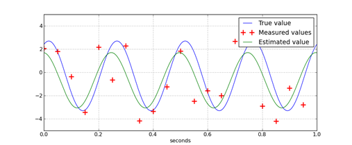
TitleGraphicsOfSineFit

If the frequency of a signal is known, the amplitude, phase, and bias on the signal can be estimated using least-squares regression. The key concept that makes this possible is the fact that a sine wave of arbitrary phase can be represented by the sum of a sin wave and a cosine wave.

image

The regression problem to find the amplitude and phase is an optimization problem. However,  it is not easily solved when using the amplitude and phase directly. This is because the problem is nonconvex; it has multiple minima.  By applying trigonometric identities, an equivalent problem, which is convex, is formed.

image

Once the regression problem is in this form, the solution is found by forming linear least squares problem. The python function illustrates how to do this. Since python’s function work in radians but most people prefer Hertz and degrees, this script performs those conversions.


from pylab import *
from math import atan2

def fitSine(tList,yList,freq):
   '''
       freq in Hz
       tList in sec
   returns
       phase in degrees
   '''
   b = matrix(yList).T
   rows = [ [sin(freq*2*pi*t), cos(freq*2*pi*t), 1] for t in tList]
   A = matrix(rows)
   (w,residuals,rank,sing_vals) = lstsq(A,b)
   phase = atan2(w[1,0],w[0,0])*180/pi
   amplitude = norm([w[0,0],w[1,0]],2)
   bias = w[2,0]
   return (phase,amplitude,bias)

if __name__=='__main__':
   import random

   tList = arange(0.0,1.0,0.001)
   tSamples = arange(0.0,1.0,0.05)
   random.seed(0.0)
   phase = 65
   amplitude = 3
   bias = -0.3
   frequency = 4
   yList = amplitude*sin(tList*frequency*2*pi+phase*pi/180.0)+bias
   ySamples = amplitude*sin(tSamples*frequency*2*pi+phase*pi/180.0)+bias
   yMeasured = [y+random.normalvariate(0,2) for y in ySamples]
   #print yList
   (phaseEst,amplitudeEst,biasEst) = fitSine(tSamples,yMeasured,frequency)
   print ('Phase estimate = %f, Amplitude estimate = %f, Bias estimate = %f'
       % (phaseEst,amplitudeEst,biasEst))
       
   yEst = amplitudeEst*sin(tList*frequency*2*pi+phaseEst*pi/180.0)+biasEst

   figure(1)
   plot(tList,yList,'b')
   plot(tSamples,yMeasured,'+r',markersize=12,markeredgewidth=2)
   plot(tList,yEst,'-g')
   xlabel('seconds')
   legend(['True value','Measured values','Estimated value'])
   grid(True)
   show()


All text is copyright © 2010, Ed Tate, All Rights Reserved.

All software and example codes are subject to the MIT License

Copyright (c) 2010, Ed Tate, Permission is hereby granted, free of charge, to any person obtaining a copy of this software and associated documentation files (the "Software"), to deal in the Software without restriction, including without limitation the rights to use, copy, modify, merge, publish, distribute, sublicense, and/or sell copies of the Software, and to permit persons to whom the Software is furnished to do so, subject to the following conditions: The above copyright notice and this permission notice shall be included in all copies or substantial portions of the Software.

THE SOFTWARE IS PROVIDED "AS IS", WITHOUT WARRANTY OF ANY KIND, EXPRESS OR IMPLIED, INCLUDING BUT NOT LIMITED TO THE WARRANTIES OF MERCHANTABILITY, FITNESS FOR A PARTICULAR PURPOSE AND NONINFRINGEMENT. IN NO EVENT SHALL THE AUTHORS OR COPYRIGHT HOLDERS BE LIABLE FOR ANY CLAIM, DAMAGES OR OTHER LIABILITY, WHETHER IN AN ACTION OF CONTRACT, TORT OR OTHERWISE, ARISING FROM, OUT OF OR IN CONNECTION WITH THE SOFTWARE OR THE USE OR OTHER DEALINGS IN THE SOFTWARE.